
Appendix: Traditional Machine Learning Foundations#
Generative AI sits on top of classical machine learning. Before a foundation model ever sees your data, someone explores it, cleans it, engineers features, turns text into numbers, and checks the result for bias. This appendix covers those foundations, exploratory data analysis, feature engineering, text processing and bag-of-words, and fairness, with short, runnable examples. It complements the generative-AI material: the text-vectorization ideas here lead directly into Tokens and Embeddings, and the fairness section reinforces Chapter 3: Dimensions of Responsible AI.
Practical companion
The hands-on labs behind these topics come from the AWS Machine Learning University
traditional-ML courses (Machine Learning through Application, and Deep Learning
Through Interactivity). The explanations and code below are original and use only
standard pandas, scikit-learn, and nltk; run the AWS lab notebooks for the
full guided exercises.
The workflow at a glance#
Classical supervised ML follows a repeatable pipeline. You explore and clean the data, engineer features, train a model, evaluate it, and check it for fairness, looping back to improve features whenever the metrics disappoint.
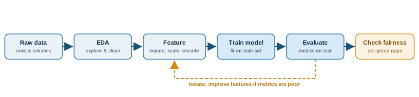
Fig. 2 The supervised machine learning pipeline. Steps run left to right; the dashed loop means you revisit feature engineering when evaluation metrics are poor.#
Background: where this sits in AI history
For decades, the accuracy of an ML system depended mostly on hand-crafted features designed by experts, the steps in sections 2-5 below. Deep learning (from roughly 2012, when a convolutional network won the ImageNet competition by a wide margin) shifted much of that work to the model, which learns features from raw pixels or text. Foundation models (from roughly 2018 onward) take this further: they pre-train once on huge data and are adapted to many tasks, the subject of this book. The classical skills here did not disappear, they are still how you understand data, build tabular models, and evaluate any system, including generative ones.
1. Working with data in pandas#
Most classical ML starts with a DataFrame: rows are samples, columns are features. The first job is simply to look at it, its shape, column types, missing values, and a few rows.
import pandas as pd

df = pd.read_csv("data.csv")
print(df.shape)          # (rows, columns)
df.info()                # column dtypes and non-null counts
df.describe(include="all")  # summary stats for numeric and categorical columns
df.isna().mean().sort_values(ascending=False)  # fraction missing per column
Knowing which columns are numerical (ages, prices) versus categorical (country, product type) determines every later step, they are explored, cleaned, and encoded differently.
2. Exploratory data analysis (EDA)#
EDA is the practice of understanding a dataset before modeling: its distributions, relationships, and quality problems. Do it well and later steps get much easier.
Categorical features#
For categorical columns you count categories and look at balance. Rare categories and high cardinality (many distinct values) both cause trouble downstream.
col = "product_category"
print(df[col].value_counts(normalize=True))     # class balance
print("distinct:", df[col].nunique())           # cardinality

import matplotlib.pyplot as plt
df[col].value_counts().head(10).plot(kind="barh")
plt.title(f"Top categories in {col}"); plt.tight_layout(); plt.show()
Numerical features#
For numerical columns you inspect the distribution (center, spread, skew) and hunt for outliers, which distort many models.
import seaborn as sns

num = "price"
print(df[num].describe())
sns.histplot(df[num], bins=40, kde=True); plt.show()
sns.boxplot(x=df[num]); plt.show()             # outliers show as points past whiskers

# correlations between numeric features
corr = df.select_dtypes("number").corr()
sns.heatmap(corr, annot=False, cmap="coolwarm"); plt.show()
Worked numerical example: the IQR outlier rule
A common, distribution-free way to flag outliers uses the interquartile range
(IQR). Suppose a price column has first quartile \(Q_1 = 20\) and third quartile
\(Q_3 = 40\), so \(\text{IQR} = Q_3 - Q_1 = 20\). The standard fences are:
lower fence = \(Q_1 - 1.5\times\text{IQR} = 20 - 30 = -10\)
upper fence = \(Q_3 + 1.5\times\text{IQR} = 40 + 30 = 70\)
Any value below -10 or above 70 is flagged as a potential outlier. A price of 250 would be well past the upper fence and worth investigating (data error, or a real but rare luxury item?). This is exactly what a box plot’s “whiskers” draw.
What to look for
Skewed distributions (long tails), heavy outliers, strongly correlated features, class imbalance, and columns that are mostly missing. Each points to a specific fix in the next step.
3. Feature engineering#
Feature engineering turns raw columns into inputs a model can learn from. The core moves:
Impute missing values (fill with a median, mode, or a learned value).
Scale numerical features so no single large-range column dominates.
Encode categorical features as numbers (one-hot for low cardinality; other schemes for high cardinality).
Create new features (ratios, dates split into parts, text length).
A scikit-learn Pipeline with a ColumnTransformer applies the right
transform to each column type and prevents data leakage by fitting only on
training data:
from sklearn.compose import ColumnTransformer
from sklearn.pipeline import Pipeline
from sklearn.impute import SimpleImputer
from sklearn.preprocessing import StandardScaler, OneHotEncoder

numeric = ["price", "age"]
categorical = ["product_category", "country"]

num_pipe = Pipeline([("impute", SimpleImputer(strategy="median")),
                     ("scale",  StandardScaler())])
cat_pipe = Pipeline([("impute", SimpleImputer(strategy="most_frequent")),
                     ("onehot", OneHotEncoder(handle_unknown="ignore"))])

pre = ColumnTransformer([("num", num_pipe, numeric),
                         ("cat", cat_pipe, categorical)])
X = pre.fit_transform(train_df)      # fit on train only, then .transform(test_df)
Why pipelines matter
Fitting a scaler or encoder on the whole dataset leaks information from the test set into training and inflates your scores. Pipelines fit transforms on the training fold only, the same discipline that matters when evaluating LLMs in Chapter 1: Evaluating LLMs.
4. Processing text#
Before text becomes features it is cleaned and tokenized. A typical pipeline lowercases, removes punctuation and stop words, and reduces words to a base form.
import re, nltk
from nltk.corpus import stopwords
from nltk.stem import WordNetLemmatizer
nltk.download("stopwords"); nltk.download("wordnet"); nltk.download("punkt")

stops = set(stopwords.words("english"))
lem = WordNetLemmatizer()

def clean(text):
    text = text.lower()
    text = re.sub(r"[^a-z\s]", " ", text)          # keep letters only
    tokens = text.split()
    tokens = [lem.lemmatize(t) for t in tokens if t not in stops and len(t) > 2]
    return tokens

print(clean("The runners were running quickly!"))
# -> ['runner', 'running', 'quickly']   (stop words removed, lemmatized)
Tokenization splits text into units (words here; subword tokens for LLMs, see Tokens and Embeddings).
Stop-word removal drops uninformative words (“the”, “is”).
Stemming / lemmatization collapses word variants (“running” -> “run”) so the model sees them as one feature.
5. Bag-of-words and TF-IDF#
The classic way to turn cleaned text into numbers is bag-of-words (BoW): build a vocabulary of all words, then represent each document by how often each word appears, order is ignored.
from sklearn.feature_extraction.text import CountVectorizer, TfidfVectorizer

docs = ["the cat sat", "the dog sat", "the cat ran"]

bow = CountVectorizer()
X_bow = bow.fit_transform(docs)          # sparse counts
print(bow.get_feature_names_out())       # ['cat' 'dog' 'ran' 'sat' 'the']
print(X_bow.toarray())                   # one row per document

# TF-IDF down-weights words common to every document (like "the")
tfidf = TfidfVectorizer()
X_tfidf = tfidf.fit_transform(docs)
TF-IDF (term frequency-inverse document frequency) improves on raw counts by scaling down words that appear in many documents and up words that are distinctive.
Worked numerical example: TF-IDF by hand
Take the three documents above and the textbook formula \(\text{tfidf}(t,d) = \text{tf}(t,d)\times \log_{10}\!\frac{N}{\text{df}(t)}\), with \(N=3\) documents and \(\text{tf}=1\) for a word present once.
First the document frequencies and IDF for each vocabulary word:
term |
df (docs with term) |
IDF = log10(3/df) |
|---|---|---|
the |
3 |
log10(1) = 0.000 |
cat |
2 |
log10(1.5) = 0.176 |
sat |
2 |
log10(1.5) = 0.176 |
dog |
1 |
log10(3) = 0.477 |
ran |
1 |
log10(3) = 0.477 |
Now the TF-IDF weights for document d1 = “the cat sat”:
term |
tf |
IDF |
tf-idf |
|---|---|---|---|
the |
1 |
0.000 |
0.000 |
cat |
1 |
0.176 |
0.176 |
sat |
1 |
0.176 |
0.176 |
The word “the” gets weight 0 because it appears in every document (it carries no
distinguishing signal), while rarer words like “dog” or “ran” would score highest.
That is exactly the behavior TF-IDF is designed for. (Note: scikit-learn’s
TfidfVectorizer uses a smoothed IDF, \(\ln\frac{1+N}{1+\text{df}}+1\), and then
L2-normalizes each row, so its numbers differ slightly but rank terms the same way.)
From bag-of-words to embeddings
BoW and TF-IDF are sparse and ignore meaning: “car” and “automobile” are unrelated dimensions. Embeddings (Tokens and Embeddings) fix this by mapping words to dense vectors where similar meanings sit close together. BoW is the historical stepping stone to the embeddings that power modern generative AI and RAG.
6. Bias and fairness in machine learning#
A model can be accurate overall yet unfair to a subgroup. Fairness work measures and mitigates that. Start by checking outcomes per group:
import pandas as pd

# y_true, y_pred are arrays; 'group' is a protected attribute column
res = pd.DataFrame({"group": group, "y": y_true, "pred": y_pred})

# selection rate (fraction predicted positive) per group
sel = res.groupby("group")["pred"].mean()
print(sel)

# demographic-parity difference: gap in selection rate between groups
print("DP difference:", sel.max() - sel.min())

# accuracy per group (a large gap is a red flag)
acc = res.assign(correct=res.y == res.pred).groupby("group")["correct"].mean()
print(acc)
Common fairness ideas:
Demographic parity: groups receive positive predictions at similar rates.
Equal opportunity: groups have similar true-positive rates.
Disparate impact: the ratio of selection rates across groups (a value far from 1 signals a problem).
Worked numerical example: is this model fair?
A hiring model is evaluated on 100 applicants from each of two groups. The confusion counts are:
group |
TP |
FP |
FN |
TN |
predicted positive |
|---|---|---|---|---|---|
A |
40 |
10 |
10 |
40 |
50 / 100 |
B |
15 |
5 |
25 |
55 |
20 / 100 |
Compute the fairness quantities:
Selection rate (fraction predicted positive): A = 50/100 = 0.50; B = 20/100 = 0.20.
Demographic-parity difference = 0.50 - 0.20 = 0.30 (large gap).
Disparate impact ratio = 0.20 / 0.50 = 0.40.
True-positive rate (recall): A = 40/(40+10) = 0.80; B = 15/(15+25) = 0.375. Equal-opportunity difference = 0.425.
By the “four-fifths rule” used in U.S. employment guidance, a disparate-impact ratio below 0.80 signals adverse impact. Here it is 0.40, well under the threshold, so despite a reasonable overall accuracy the model treats group B markedly worse and would need mitigation.
Mitigations act at three stages: pre-processing (reweight or rebalance the data), in-processing (add fairness constraints during training), and post-processing (adjust decision thresholds per group). This is the concrete, tabular-ML counterpart of the fairness dimension in Chapter 3: Dimensions of Responsible AI, and the same care applies to generative models.
Recent developments and tooling#
The classical workflow is increasingly automated and audited:
AutoML tools (such as AWS AutoGluon, and others like auto-sklearn and H2O) automate model selection, feature preprocessing, and hyperparameter tuning, often training and ensembling many models with a few lines of code. They make strong tabular baselines accessible without deep expertise.
Fairness toolkits such as Fairlearn and AIF360 provide standard metrics (demographic parity, equal opportunity) and mitigation algorithms, so the hand computations above become one function call, and are auditable.
Text has largely moved from sparse to dense. Bag-of-words and TF-IDF are still excellent baselines, but most modern NLP replaces them with contextual embeddings from transformers, the bridge into this book’s generative-AI chapters (Tokens and Embeddings, Chapter 3: Retrieval-Augmented Generation).
Responsible-AI regulation (the NIST AI RMF and others in Chapter 2: Foundations of Responsible AI) increasingly expects the bias checks in section 6 to be documented, not optional.
Knowledge check#
Test your understanding. Each answer is hidden, click to reveal.
Q1. Why fit a scaler or encoder on the training set only?
Fitting on the full dataset lets information from the test set (its means, scales, categories) leak into training. That inflates evaluation scores and overstates how well the model will generalize. Pipelines fit on the training fold and only transform the test fold.
Q2. In the TF-IDF example, why does “the” get a weight of zero?
“the” appears in all \(N=3\) documents, so its document frequency is 3 and its IDF is \(\log_{10}(3/3)=\log_{10}(1)=0\). Multiplying any term frequency by 0 gives 0: words common to every document carry no distinguishing information.
Q3. A model has 92% overall accuracy but a disparate-impact ratio of 0.55. Is it fine to deploy?
No. A disparate-impact ratio of 0.55 is below the 0.80 “four-fifths” threshold, indicating the model selects one group far less often than another. High overall accuracy can hide serious per-group harm, which is why fairness is measured per group, not just in aggregate.
Q4. What is the main limitation of bag-of-words that embeddings fix?
Bag-of-words is sparse and treats every word as an independent dimension, so “car” and “automobile” are unrelated. Embeddings map words to dense vectors where similar meanings are close together, capturing semantic relationships that BoW cannot.
Q5. Using the IQR rule with Q1 = 30 and Q3 = 50, is a value of 95 an outlier?
IQR = 50 - 30 = 20. Upper fence = \(Q_3 + 1.5\times 20 = 50 + 30 = 80\). Since \(95 > 80\), yes, 95 is flagged as a potential outlier.
Key takeaways#
Classical ML begins with EDA: understand distributions, cardinality, correlations, and data-quality issues before modeling.
Feature engineering (impute, scale, encode, create) via leak-safe pipelines turns raw columns into model inputs.
Text is cleaned and tokenized, then vectorized with bag-of-words / TF-IDF, the sparse ancestors of dense embeddings.
Fairness is measured per group (parity, equal opportunity, disparate impact) and mitigated at the pre-, in-, or post-processing stage.
These foundations underpin everything generative AI does; the vectorization and fairness threads connect directly to Tokens and Embeddings and Module 2.